Quadratics and rate-of-change functions
Background
Shannon and the students are working on a unit of quadratics and rate of
change functions. On the first day of the unit, the class looked at a
constant rate of change function, and constructed the linear function that
has that rate of change. Then the students were asked to repeat the exercise
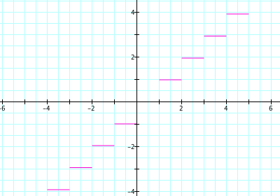
with a rate of change function that was a step function of step size 1 that
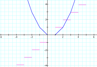
approximated a line. Their result was a piecewise linear approximation to a
quadratic curve. Shannon used graphing calculator to demonstrate how smaller
and smaller intervals would produce a smoother looking curve.
Figure 1: A rate of change step function produces a
piecewise linear 'original' function.


A Classroom moment
This is a clip from the second day of the unit. Prior to this clip, the
students have been given a graph of the function x2 on grid
paper. The students have been asked to fill in a table by going through the
graph in intervals of step size one, and calculating the average rate of
change of the graph for each interval. Average rate of change was not a new
idea to the students. It had been discussed in prior units. Each row of the
table consists of the end points of the interval and the rate of change for
that interval.
| Start Point |
End Point |
Avg. Rate of Change |
| (-4, 16) |
(-3, 9) |
-7 |
| (-3, 9) |
(-2, 4) |
-5 |
| (-2, 4) |
(-1, 1) |
-3 |
| (-1, 1) |
(0,0) |
-1 |
| (0,0) |
(1,1) |
1 |
| (1,1) |
(2,4) |
3 |
| (2,4) |
(3,9) |
5 |
| (3,9) |
(4,16) |
7 |
In this clip, Shannon asks the students to graph the results on their
table. Specifically, she asks them to "graph the rate of change on the y
axis... with their corresponding x values. But see how this rate of change
has two corresponding x values? Take the left one."
Looking at student work
As Shannon moves from student to student, she notices that some students
have sketched step functions and others plotted a series of points. Few
students did as she anticipated -- plot the points and then connect them.
The students' graphs are actually a welcome, even if unanticipated,
development. Those students who drew step functions seemed to have thought
about the function's rate of change at values within the interval and used
the best information they had -- that it didn't change (hence a constant
function over each interval). Those students who plotted points seemed to
see no reason to go beyond the information given -- meaning that no
information was given about the rates within the intervals, so they
couldn't sketch anything.
Discussing students' work
Shannon called the class together to discuss their reasoning for the
graphs they sketched, and to discuss how to construct a more accurate
graph for the original function.
A Follow-up Interview
Shannon had not anticipated that students would graph step functions in
their answers. Rather, she had expected that the students would connect
their plotted points to form a line. As the video above shows, several
students did not connect the points: either leaving them as points, or
graphing a step function.
Two days later, in this follow up interview, Sharon and Carlos ask one of
the students about his choices to graph a step function. Caution: the audio
is much louder for this clip

