|
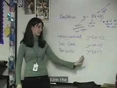
Ms. Coombs begins with a reminder of an
earlier problem about a pie eating
contest. She discusses the meaning of
the elements of a linear function. This
discussion follows her working to interpret
y=mx+b style equations with the
students.
|
|
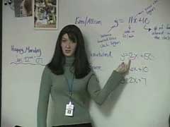
In this clip Ms. Coombs continues the
discussion by asking about constant
rates. She steers the discussion
towards constant speed and the rates in the
linear functions.
|
|
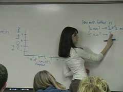
Ms. Coombs continues to focus on the earlier
pie eating function. In this clip, she
moves to a graphical representation for the
function. In order to tie back into
covaritational thinking she reminds the
students about the finger tool. She
generates points on the graph by
covariationally scaling the rate.
|

|
In this clip Ms. Coombs works with the
students to focus on the possible points
between plotted points on the graph of the
linear function. She explains why the
intermediate points exist and why those
points lie on the line. She focuses on
how changes in x determine the changes in y,
based on the rate of change.
|
|
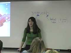
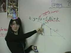
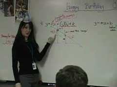
Having now familiarized students with the
y=mx+b form and reminding the students to
think covariationaly, Ms. Coombs introduces
a problem to serve as a point of ongoing
discussion to develop another form for
linear functions – one that allows for
finding an equation when given a point and a
rate of change. The problem states
that Ms. Coombs checked her watch 7 minutes
ago when she was 3.8 miles from home.
She also knows she is traveling at ½ mile
per minute. In this clip Ms. Coombs
asks the students to model this on a
graph. One student volunteers to
provide the graph.
|
|
Ms. Coombs continues with the discussion,
but she also includes the information that
she was traveling at ½ mile per
minute. She asks how far she will have
traveled in ½ of a minute. Ms. Coombs
then asks about other fractions of
additional times and the corresponding
changes in distances.
|
|
In this clip Ms. Coombs continues to develop
the traveling problem from the day
before. She uses a table to help
organize not just the changes, but also the
overall distance traveled. This
discussion depends on her rate of
change. She works with the students to
find her distance seven minutes before she
checked her watch.
|
|
Building from the earlier ideas, in this
clip Ms. Coombs asks about changes in
y for given changes in
x after revisiting the linear form
y=mx+b. She focuses on multiplying the
change in x by the rate of change
to find the resulting change in y.
|

|
The students use the graphing calculator
program to solve the problem of finding the
equation of a line with a rate of change of
-2 passing through the point (-3,4). In this
case x increases by 3 so
y changes by “negative 2 times as
much.” Ms. Coombs then reminds
students where the function is changing
from. In essence, the
students know the -2x, they are working
covariationally to find b.
|
|
Prior to this clip, students were given the
point (5, 2) with the rate of change -7 and
asked to find the corresponding linear
function using the graphing calculator
program. Here, we see Ms. Coombs
working with a pair of students to determine
the initial value, b, by
coordinating the change in x with a
change in y. In this process
students struggle with the meaning behind
what has become a mantra of “y changes by
___ times as much.”
|
|
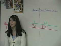
Ms. Coombs then introduces a chart in which
she records all of the little changes that
the students determined the previous day.
For example, how much did her distance from
home change in 7.1 minutes versus in seven
minutes. The conversation then changes to
determining where Ms. Coombs was when she
started her watch or at zero minutes. In
this process, she is continually re-visiting
constant rate of change.
|
|
Later, Ms. Coombs continues with having
students reason about how the two variables
in a linear function change with respect to
each other. In particular, she relates a
change in x to a change in y.
|
|
Later, Ms. Coombs continues with having
students reason about how the two variables
in a linear function change with respect to
each other. In particular, she relates a
change in x to a change in y.
|
