 |
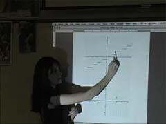
In this first clip we see Ms. Coombs focus students’ attention on rate of change. She begins by having the students consider a problem:
|
 |
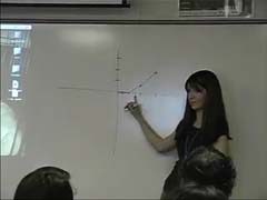
Ms Coombs continues to work through the earlier task. She considers how the rate of change information will translate to the original function by considering intervals to the right of x = 0.
|
 |
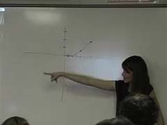
After giving students time to work on the problem, Ms. Coombs continues the discussion of the rate of change step function. She uses her earlier proportional rate language where y changes by some amount that is “times as much” as the change in x. The focus of this clip is for x < 0 on the domain.
|
 |
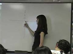
Ms. Coombs leads the class in thinking about the impact of changing the step interval on the rate of change graph from 1 to ½ units. To do so she provides a graph of this new step function. Students reach the conclusion that the resulting graph will be “more specific.”
|
 |
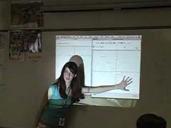
In this clip, Ms. Coombs asks students what they meant by “more specific.” She leads into this question by pushing the step size down to 0.1 units. Additionally, Ms. Coombs directs the class in a discussion about the implications these smaller step sizes have on the resulting graph.
|
 |
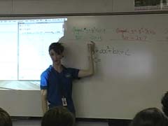
Ms. Coombs asks students to make a connection between the previously learned distributive property and the current topic of binomial multiplication. Students assign the placeholders a, b, and c from (a+b)c = ac + bc to the example y = (x + 4)(x + 6). She leads the class through the distributive process twice in order to write the binomial product in the expanded, quadratic form.
|
 |
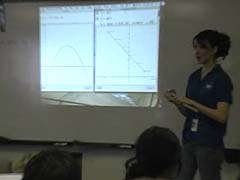
Using the Graphing Calculator software, Ms. Coombs shows students what happens to the graph of an original function when the step size decreases on its corresponding rate of change graph.
|
 |
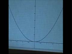
In this clip, Ms. Coombs reverses the earlier activity and now gives students the graph of y = x2 and asks them to sketch a graph of its corresponding rate of change function. In this clip the students begin by working with intervals of one unit.
|
 |
In this clip Ms Coombs guides the class to discuss their computed rates of change for unit length intervals on y = x2. Once she is sure that all of the students agree on the numeric results, she asks them to graph the rate of change values as a function of x.
|
 |
In this clip, we see the work of several students after they create the graph of the rate of change function. She continues the discussion by asking students how they could make the rate graph more accurate.
|
 |
Ms Coombs works with the students on graphing the rate of change function for
y = -(x2). In this task it is evident that students have a difficult time thinking about a function with negative values and a positive rate of change.
|
 |
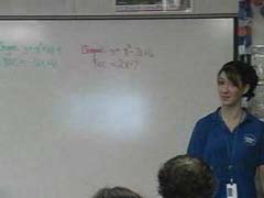
In an earlier discussion Ms Coombs had the students find the equation of the line that connected the left points of each step of the rate of change step function. She also had them find the equation of the line connecting the right end points of each step of the step function. In an effort to find the “accurate” line, the students then found the line in-between the two functions. In this clip Ms. Coombs reviews this process. The function is y = -(x2) + 6x - 4. The function connecting the left end of each rate of change step function is y = -2x + 5. The function connecting the right end of each step is y = -2x + 7. Ms Coombs uses the graphing calculator program to show the “accurate” equation to be y = -2x + 6.
|
 |
In this clip, Ms. Coombs reviews the pattern for determining a rate of change function from a given quadratic function.
|
 |
Ms Coombs continues to discuss the pattern to find the rate of change function for a given quadratic function. Here, she presents the function in the generalized form
y = ax2 + bx +c. The students disagree over the answer.
|
 |
Ms Coombs now works with a continuous rate of change function rather than a step function. Here, she leads the class in discussing how the graph of a function will behave given a continuous, linear rate of change graph.
|
 |
The students now need to focus on the significance of the zero on the linear rate of change function. In this clip, Ms. Coombs works with a student to help her identify the x-value of the vertex of the graph of a quadratic function given the graph of its rate of change function.
|
 |
On the worksheet seen in this clip the students are given a quadratic function and the rate of change function. The students are asked to graph the rate of change function, and then to graph the quadratic. In this clip, Ms Coombs works with a student to focus on the x intercept of the rate of change function.
|
 |
In this clip, a student explains her understanding of the relationship between the graph of a linear rate of change function and the vertex of its corresponding quadratic function. In this task, the given quadratic is y = -2x2 + 4x + 5, the rate of change graph is y = -4x + 4, and the vertex is at x = 1.
|
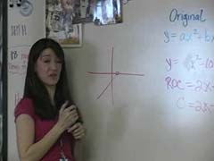 |
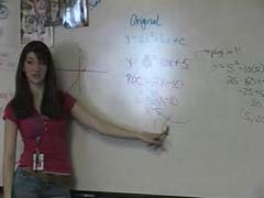
Ms. Coombs leads the class through the process of finding the x and y values for the vertex of a given quadratic function, y = x2 - 10x + 5. She finds the vertex using the rate of change function.
|
 |
Ms Coombs continues the discussion by focusing on how a vertex of a quadratic can represent a maximum or minimum. One student’s explanation focuses exclusively on working from an imagined graph of the rate of change function.
|
